Mapping the Intestinal Social Network using Data

Download the full research paper (PDF)

This is a friendly walk through of how linear algebra, random walks and consensus statistics uncover who talks to whom inside the mouse gut. Thanks to all of Group 19 for the joint-effort on this!

---

1 Understanding the Bio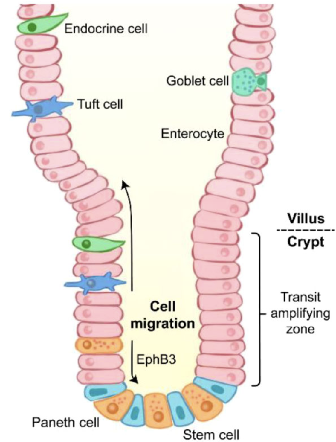

Stem cells live at the bottom of each intestinal crypt, crank out transient‑amplifying daughters, and those daughters sprint up the villus to become one of several mature cell types (enterocytes, goblets, Paneth, Tuft, …).
Biologists know that story; here we’ll focus on how the data science works behind the scenes.

Our raw material: a single‑cell RNA‑seq cohort (≈ 5 000 cells, ~24 000 genes) capturing the full crypt‑to‑villus journey.

---

2 From a 24000 Dimension gene space to a colourful UMAP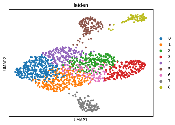

2.1 k‑NN + Leiden ≥ k‑means

1. Dimensionality crunch. PCA keeps the top d = 50 principal components.
2. Graph build. For each cell i, find its k=15 nearest neighbours under Euclidean distance in PC‑space.
3. Edge weights. Use the Jaccard index so shared neighbourhoods matter more than raw distance.
4. Leiden partitions the graph by maximising modularity

\[Q=\frac{1}{2m}\sum_{ij}\Bigl(A_{ij}-\tfrac{k_i k_j}{2m}\Bigr)\delta(c_i,c_j)\]

with an extra “refinement” phase that guarantees well‑connected clusters.

Result: nine clearly separated communities.

2.2 First‑pass labels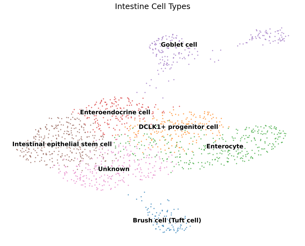

Marker genes (e.g. Lgr5, Muc2, Defa) give us a draft taxonomy: ISC, TA, Paneth, Goblet, Enteroendocrine (EEC), Tuft, …

2.3 Tightening the taxonomy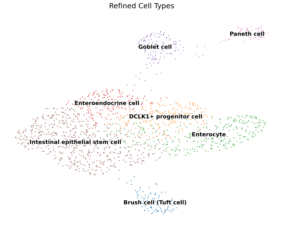

A second Leiden round on each broad group + differential‑expression tests cleans up stragglers — leaving a high‑confidence cast of seven major players.

---

3 A summary of ligand–receptor maths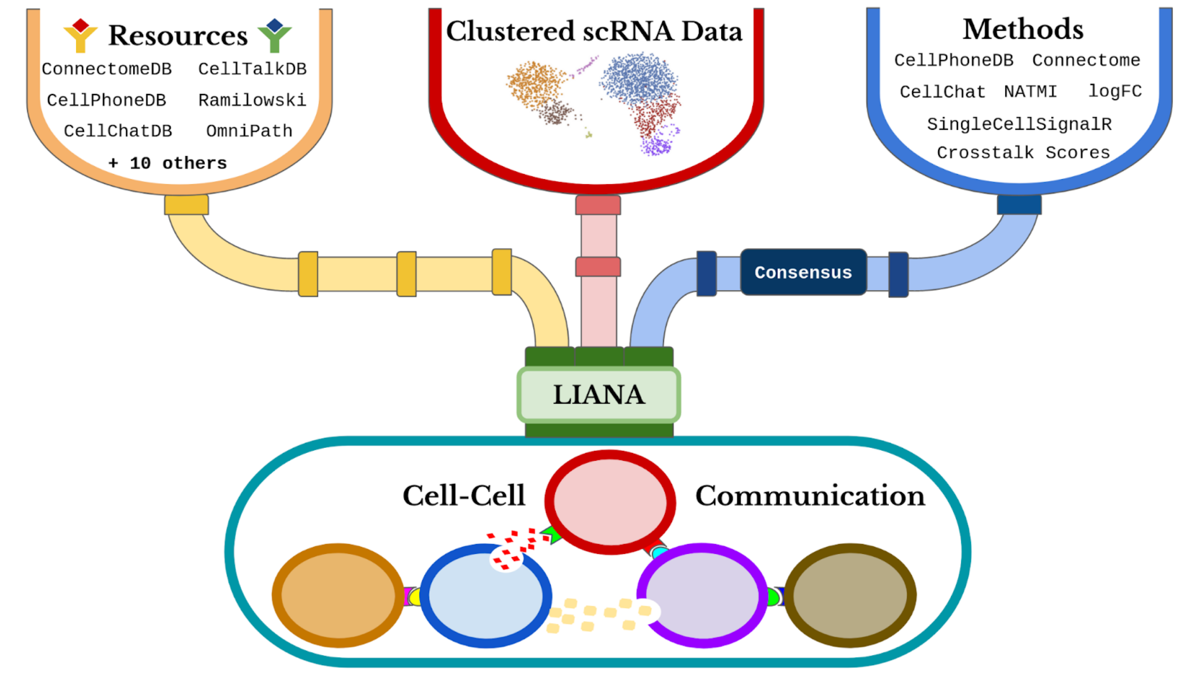

Instead of betting on a single L‑R scoring scheme, LIANA pipes our clustered counts into six independent algorithms (CellPhoneDB, NATMI, logFC, …) and spits out a consensus z‑score per sender/receiver pair.

Mathematically it’s just:

\[z_{sr}=\frac{1}{M}\sum_{m=1}^{M}\frac{s_{sr}^{(m)}-\mu_m}{\sigma_m}\]

— i.e. average the method‑specific z‑scores so no method can single‑handedly skew the ranking.

---

4 Static interaction analysis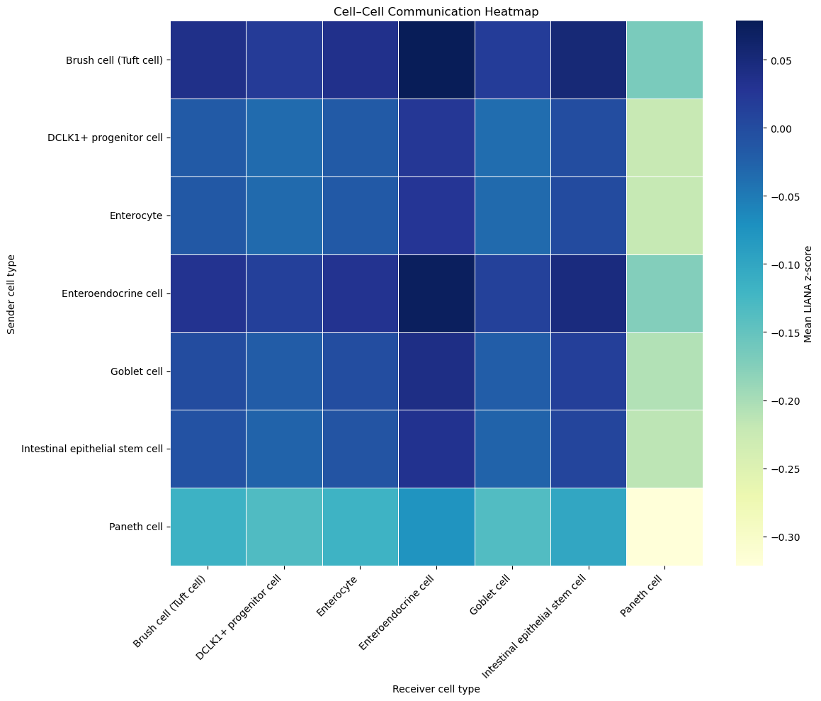

Rows = senders, columns = receivers, colour = mean LIANA z‑score (blue → positive, yellow → negative).

• Observations worth flagging:
  • EECs broadcast like crazy — they top almost every column.
  • Paneth cells are selective but punchy (strong blue into ISCs, neutral elsewhere).
  • Self‑loops (diagonal) aren’t always dominant; Goblets talk more to Paneth than to themselves.

How is the heatmap built? Just stack all individual L‑R pairs, compute the sender‑receiver‑averaged z‑score, then visualise the matrix.

---

5 Random walks through pseudotime

5.1 Diffusion pseudotime summary

• Construct the diffusion kernel $K=\exp(-D^2/\sigma)$ from the PC‑space distances $D$.
• Normalise rows → Markov matrix $P$.
• Pseudotime of cell i is the diffusive distance to the root:

\[\operatorname{dpt}(i)=\sum_{l=2}^\infty\lambda_l^{-1}(e_i-u)^\top\psi_l\]

where $\lambda_l,\psi_l$ are eigen‑pairs of $P$ and $u$ is the stationary vector.
That score is then binned into ten equal‑width intervals Bin 0…9.

5.2 Heatmaps per bin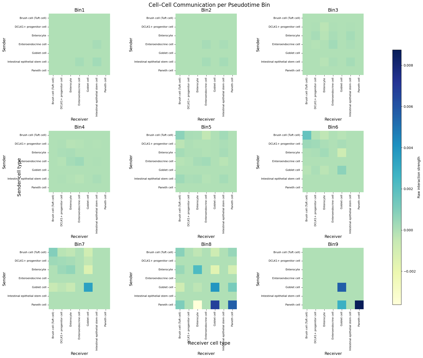

Each 3 × 3 panel speaks a short sentence:
“Who’s signalling right now?”
Early bins are almost silent. Starting Bin 6, Paneth → Paneth and Goblet → Goblet squares glow blue, hinting at lineage‑restricted chatter as cells mature.

5.3 Quantifying the trends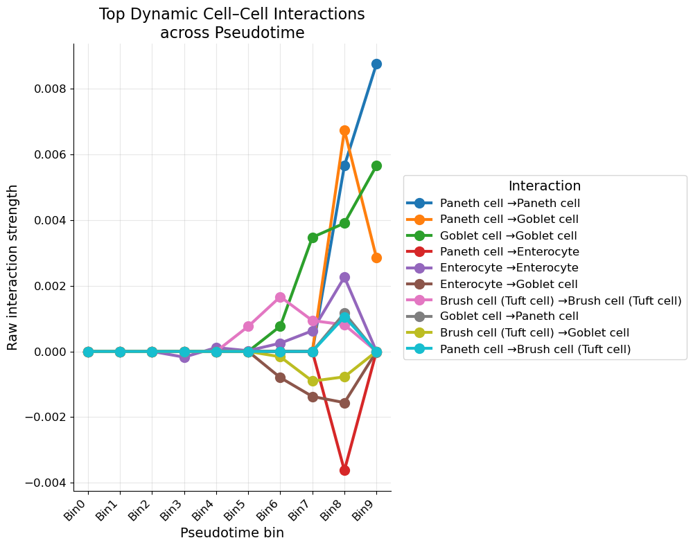

For every sender/receiver combo we regress raw LIANA score against bin index and keep the ten steepest slopes.
Take‑away maths:

• Slope $>0$ ⇒ interaction ramps up along differentiation;
• Slope $<0$ ⇒ ramps down;
• $R^2$ values hover 0.6‑0.9, so the linear fit is not shabby.

Paneth → Paneth tops the chart (slope ≈ 8 × 10⁻³), reinforcing the idea of a self‑reinforcing niche late in crypt life.

---

6 Wet‑lab validation

Paneth niche drives budding

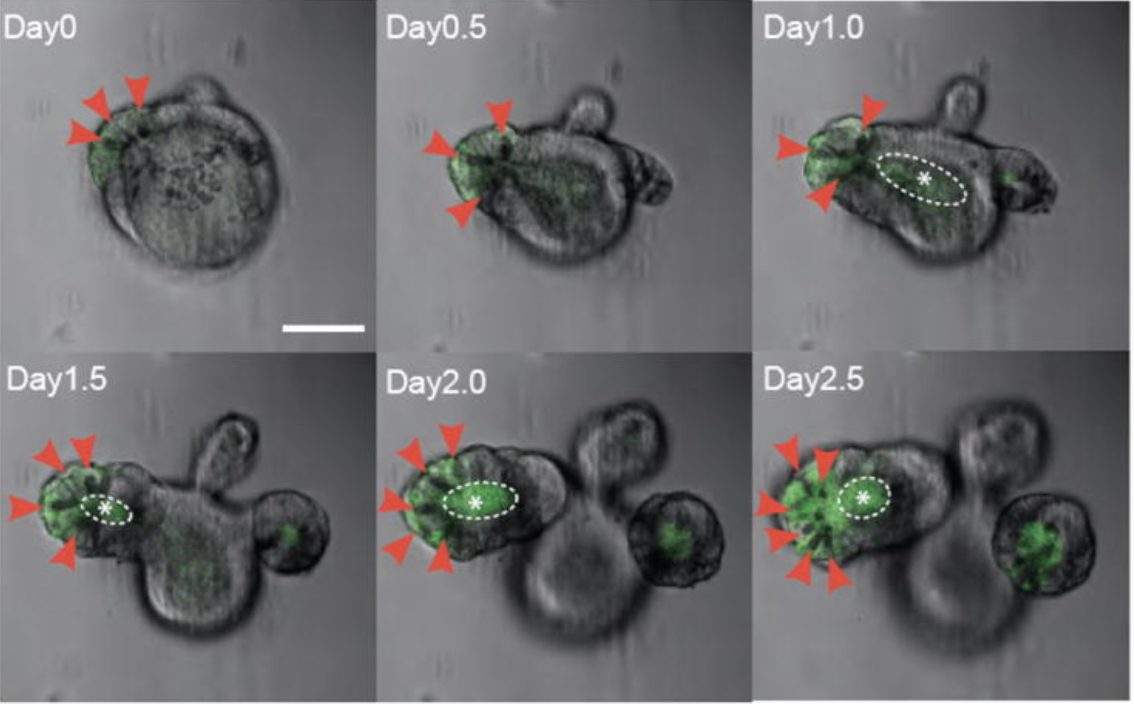
Evidence: Live imaging shows crypts sprout exactly where a Paneth cell (green, red triangles) contacts ISCs (white asterisk). Frames map almost 1:1 onto Paneth → ISC spike in Bin 7‑9.

EECs modulate organism‑level metabolism

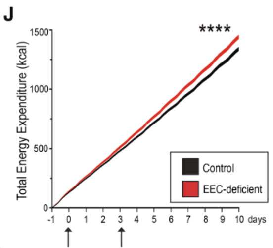
Evidence: Knock‑out of EECs ⇒ mice burn *extra* calories (red line). High EEC → Global signaling in complete heatmap predicted they're key metabolic broadcasters.

---

7 Conclusion — the maths is portable

1. Graph theory (Leiden, k‑NN) finds the cast.
2. Spectral kernels (Diffusion map) supply a clock.
3. Markov chains (random walks on the interaction graph) estimate fate probabilities — we skipped the CellRank details here, but it’s essentially solving $(I-Q)^{-1}R$.
4. Ensemble statistics (LIANA consensus) damp idiosyncratic bias.

Swap out mouse gut for tumour micro‑environment or developing retina and the pipeline survives intact.

---

For further details, see the attached PDF or contact the author for discussion.

Share this post