Mean-Field Market Making
Introduction
I was reading Terry Tao’s blog the recently and stumbled across this pretty cool field of maths: Mean Field Games. It’s like if game theory and stochastic differential equations had a kid and its fairly new as well. He has some amazing analogies at the start of his blog which I hope he wont mind me copying (he will never see this blog page) to better explain the ideas of Mean Field Games to sort of set the scene for you.
Some intuition on Mean Field Games
You’ve probably been to some sort of stadium in your life (if you haven’t then Ctrl+W right now and go book tickets for some random sporting fixture). Mexican Waves are one of those things that most people want to do but a lot of just don’t have the guts to start off that chain in the event of horrific failure and consequential embarrasment. At some point in our life, we have all pondered - “how do we determine our effort and response to the Mexican Wave headed our way.”
Well, ignoring pyschologists and biologists exist, it definitely makes sense to turn to the mathematician and leave it to them to turn a person into a function with parameters that satisfy some (stochastic) differential equation. What this might leave us with is a scenario in which this effort and response to the wave is governed by some differential equations over a “Mean” (hopefully its clicking now), where the mean is a large number of other “players” of this game. What we ask ourselves is: based on our own functions and parameters such as confidence or response of nearby agents, what is our best response in this game?
From Mexican Waves to Market Making
Market Making is something which I was first exposed to at a spring week I did at Optiver. It took some time to get my head around during that spring week but I managed to understand the general idea behind it after being shouted at multiple times - “YOU CANT BUY A BID!”
I’ll have a go at explaining market making as best I can with setting the scene of another super common life experience, a bustling fruit market that only sells apples with lots of stalls and lots of customers. In the market place, we consider what the best “ask” of a farmer (seller) is and the best “bid” of an apple buyer is. Intuitively, if these prices lineup/overlap, trades will take place (think someone is selling something for £50 but you are willing to pay £60, you will obviously buy). However, when these prices don’t line up and the spread between the two increases more and more, we face a problem called “illiquidity”. Trades aren’t happening in this marketplace and its neither good for the farmers nor the customers.
What a market maker (mm) will come and do is tighten that bid-ask spread to provide liquidity to the market to encourage trading and as a result profit on the spread of their bid and ask. A quick example may help to demonstrate this:
No Market Maker Present: Best Ask: £8 a crate, Best Bid: £5 a crate. Result: Super low level of trading
Market Maker Present: MM Ask: £7 a crate, MM Bid: £6 a crate. Result: More trading, market maker profits on £1 spread.
The Aim of the Project
Issues with traditional systems
Many of the current models used in market making such as Avellaneda–Stoikov (I’ll write a blog about this soon!) assume you are the only agent, you end up optimising your quotes based on exogenous flow (in the apple analogy this translates to “the number of shoppers walking past each minute is fixed by the weather,regardless of how stalls set prices”). In reality, markets witness more endogenous flow: “if all apple stalls cut prices, shoppers run to the cheapest vendors, changing your foot traffic.”
Another issue is scalability, simulating hundreds of interacting makers as an N-player stochastic game is intractable; single-agent models can’t capture the feedback loop and N-player models don’t scale reasonably.
Why is adding Mean Field Games so good?
Mean Field Games (MFG) treats a continuum of small players and treats everyone else with a mean field - this is the distribution of inventories and average quotes.
MFG uses two coupled equations: Hamilton-Jacobi-Bellman (HJB) and Fokker Plank (FP) to capture the loop between making new quotes based on the evolution of other makers distribution.
From a broad angle, the mechanics of the two equations are as follows:
- HJB (backward): each maker’s optimal quotes given the crowd.
- Fokker–Planck (forward): how the crowd distribution evolves when everyone follows those quotes.
Solving these equations for their fixed point gives you:
- Endogenous intensities: fill rates depend on your relative tightness to the crowd average—exactly the competitive mechanism.
- Equilibrium spreads: a time-path for the population’s bid/ask behavior (when spreads naturally compress or widen).
- Crowd inventory dynamics: when de-risking waves happen, how concentrated inventory becomes, who is likely stuck at the bell.
In a world where algorithmic tradings tumps manual trading, ignoring feedback from interacting strategies creates systematically biased expectations for trades, PnL and risk.
The aim of this project is to implement this theory in the world of market making to hopefully create a system which provides optimal quotes based on the market’s trading itself - without us actually knowing what the market is trading and is about.
Below is a quick overview of what we found - mainly for those who don’t want to get their hands dirty in the maths and only in results:
Over a trading day $[0,T]$, our solver computes:
- a value function $V(t,x)$ — the best expected objective you can still achieve from time $t$ with inventory $x$
- optimal bid $\delta^{b*}(t,x)$
- optimal ask $\delta^{a*}(t,x)$
- the evolving population distribution $\rho(t,x)$ of inventories;
- actionable metrics such as average bid/ask, full spread, inventory variance, de-risk probability, and marginal cost.
The interactive dashboard below renders the same objects the solver computes.
Interactive Value Function Preview
3D Value Function Preview: Shows how V(t,x) evolves over time and inventory
Interactive Demos
Throughout this post, you’ll find interactive visualizations that bring the mathematical concepts to life. Each demo focuses on different aspects of the mean field games market making model.
Main Dashboard
Main Dashboard: Overview of all key metrics and dynamics
Modelling the Bid-Ask Spread
Lets go back to the apple market. Imagine that a big board shows the current mid price of the apples. As a market maker, you want to set two prices relative to that mid:
- ask markup $\delta^a_t \ge 0$ (how far above mid you sell one unit),
- bid markdown $\delta^b_t \ge 0$ (how far below mid you buy one unit).
Spread identity (sign convention used here). With ask $\ge 0$ and bid $\le 0$, \(\text{Full spread} \;=\; \delta^a_t + \delta^b_t \;=\; (m_t + \delta^a_t) \;-\; (m_t - \delta^b_t) \;=\; \text{ask} \;-\; \text{bid}.\)
Intuitively: tighter prices (smaller $\delta$) attract customers; wider prices discourage them from trading.
We can model trades at our quotes with Poisson processes. The intensity (rate) falls off exponentially with the distance from mid-price. This is standard, simple, and empirically reasonable: \(\lambda^a(\delta) \;=\; A\,e^{-k\delta}, \qquad \lambda^b(\delta) \;=\; A\,e^{-k\delta}, \qquad A>0,\; k>0.\)
- $\lambda$ is a rate: expected fills per unit time.
- If you tighten by $\Delta\delta>0$, the relative change in rate is: \(\frac{\lambda(\delta-\Delta\delta)}{\lambda(\delta)} \;=\; e^{k\,\Delta\delta}.\)
Inventory $X_t$ changes by single-unit jumps:
- ask fill (you sell) makes $X \to X-1$,
- bid fill (you buy) makes $X \to X+1$.
We use edge accounting relative to mid: a sell at $\mathrm{mid}+\delta^a$ earns edge $\delta^a$; a buy at $\mathrm{mid}-\delta^b$ also earns edge $\delta^b$. Mid cancels from the accounting.
Edge vs Inventory Risk
If you have apples at the end of the day, they might go bad overnight or maybe the orange market sees literal overnight success, reducing demand significantly for apples.
Similarly, market makers may try and finish close to a neutral position by market close: this is definitely not always true but this strategy certainly helps reduce risk.
During the day you accumulate an edge when trades occur, pay a running cost for carrying inventory, and care about ending flat. Assume we have some policy $\pi$ such that: \(J^\pi(t,x) = \mathbb{E}_{t,x}^{\pi}\!\left[ \int_{t}^{T} \big( \delta^a_s\,dN^a_s + \delta^b_s\,dN^b_s - \eta\,X_s^2\,ds \big) \;-\; \gamma\,X_T^2 \right].\)
- $dN^a_s$ and $dN^b_s$ are Poisson increments,
- $\eta>0$ penalizes intra-day inventory,
- $\gamma>0$ penalizes terminal inventory (overnight risk, closing dumps, etc.).
The value function is the best you can do from $(t,x)$: \(V(t,x) \;=\; \sup_{\pi} J^\pi(t,x).\)
You can think of this as: “from now until close, what’s the maximum expected ‘edge minus risk’ I can still achieve if I currently hold $x$ crates?”
From dynamic programming to the HJB
Consider a small shift in time $h>0$. Three outcomes can happen over $[t,t+h]$:
- ask fill with probability $\lambda^a(\delta^a_t)\,h + o(h)$: reward $\delta^a_t$, inventory $x\to x-1$;
- bid fill with probability $\lambda^b(\delta^b_t)\,h + o(h)$: reward $\delta^b_t$, inventory $x\to x+1$;
- no fill with probability $1-(\lambda^a+\lambda^b)h + o(h)$.
Running cost over that interval is approximately $-\eta\,x^2 h$. We utilise the Dynamic Programming Principle to give:
\[V(t,x) = \sup_{\delta^a,\delta^b} \mathbb{E}\!\left[ \int_{t}^{t+h} \bigl(\delta^a_s\,dN^a_s + \delta^b_s\,dN^b_s - \eta\,x^2\,ds\bigr) + V\bigl(t+h, X_{t+h}\bigr) \right] + o(h).\]Expand $V(t+h,\cdot) = V(t,\cdot) + \partial_t V(t,\cdot)\,h + o(h)$. Take expectations, subtract $V(t,x)$, divide by $h$, and let $h\to 0$. The Hamilton–Jacobi–Bellman (HJB) equation is: \(-\partial_t V(t,x) = \sup_{\delta^a,\delta^b} \Big\{ \lambda^a(\delta^a)\,[\delta^a + V(t,x-1) - V(t,x)] + \lambda^b(\delta^b)\,[\delta^b + V(t,x+1) - V(t,x)] - \eta\,x^2 \Big\},\) \(V(T,x) \;=\; -\gamma\,x^2.\)
We can interpret each bracket as the “instant edge plus change in future value, weighted by how likely that trade is right now.”
Optimal quotes in closed form
Inside the HJB, each side can be optimized separately. For the ask side, let $\Delta V^a(t,x)=V(t,x-1)-V(t,x)$. We maximize: \(f(\delta) \;=\; \lambda(\delta)\,[\Delta V^a + \delta] \;=\; A\,e^{-k\delta}\big(\Delta V^a + \delta\big).\)
Differentiate and set equal to $0$: \(f'(\delta) \;=\; A\,e^{-k\delta}\,\big[-k(\Delta V^a+\delta) + 1\big] \;=\; 0 \quad\Rightarrow\quad \delta^{a*}(t,x) \;=\; \frac{1}{k} \;-\; \big[V(t,x-1) - V(t,x)\big].\)
Subject to non-negativity: if the right-hand side is negative, set $\delta^{a}=0$. The same applies to $\delta^{b}$.
Our bid is analogous: \(\delta^{b*}(t,x) \;=\; \frac{1}{k} \;-\; \big[V(t,x+1) - V(t,x)\big].\)
If selling is urgent (you are long near close), $V(t,x-1)-V(t,x)$ is very negative, so $\delta^{a *}$ becomes small — you tighten to get hit. If buying back is urgent (you are short), $\delta^{b *}$ shrinks too. In our code we clipped $\delta$ to practical bounds.
\[\delta^{a*} \;=\; \frac{1}{k}\;-\;\bigl[V(t,x-1)-V(t,x)\bigr].\]Interactive Control Surfaces
Optimal Control Surfaces: Shows how δ*(t,x) varies with time and inventory
Ask Control Surface: Optimal ask spreads δ^a*(t,x)
Bid Control Surface: Optimal bid spreads δ^b*(t,x)
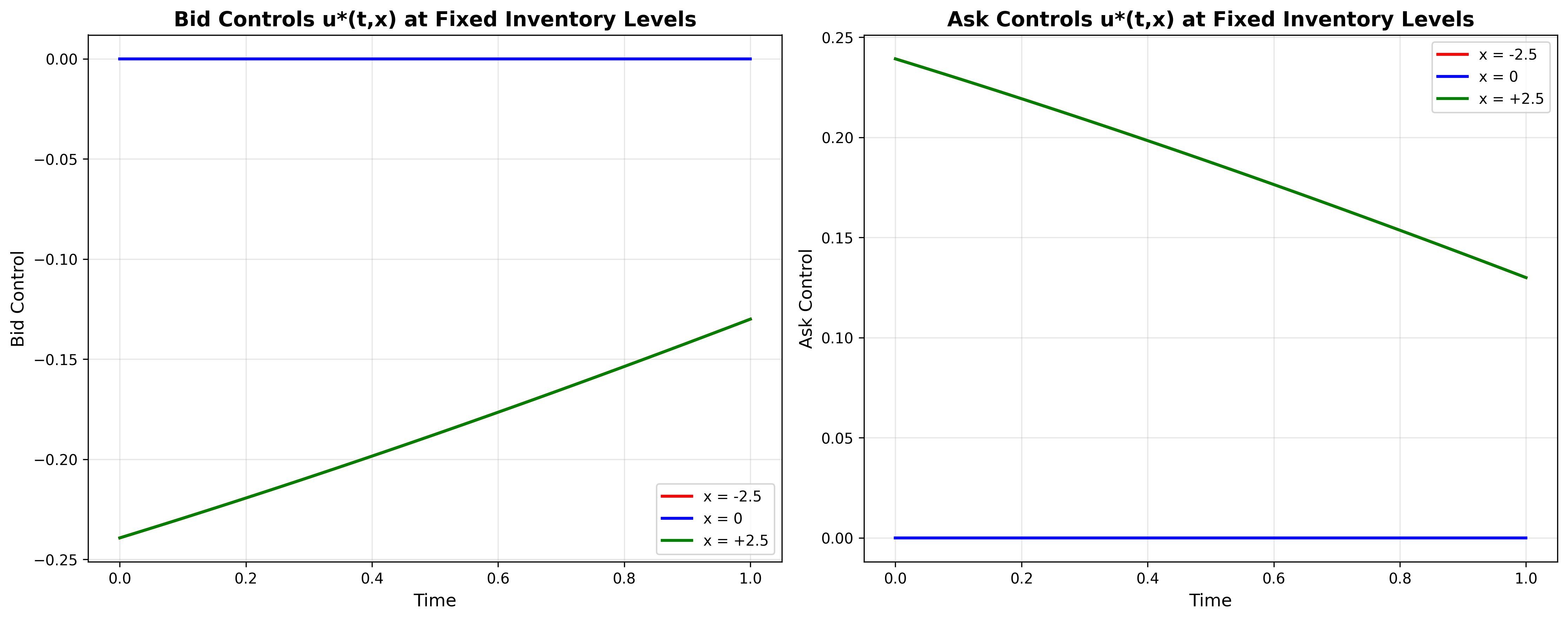
Control Slices: Cross-sectional views of optimal spreads at different times and inventory levels
Everyone Else: Fokker–Planck
Let $\rho(t,x)$ be the fraction of makers at inventory $x$ and time $t$. Under the optimal quotes: \(\partial_t \rho(t,x) = \rho(t,x+1)\,\lambda^a\!\big(\delta^{a*}(t,x+1)\big) + \rho(t,x-1)\,\lambda^b\!\big(\delta^{b*}(t,x-1)\big) - \rho(t,x)\,\big[\lambda^a\!\big(\delta^{a*}(t,x)\big) + \lambda^b\!\big(\delta^{b*}(t,x)\big)\big].\)
This is a mass balance inflow from neighbors that trade into $x$ minus outflow from $x$ that trade away.
Probabilities sum to one at each time: $\sum_x \rho(t,x)=1$.
The de-risk probability used in the charts is: \(P\big(|X_t|<\varepsilon\big) \;=\; \sum_{|x|<\varepsilon} \rho(t,x)\) (where the sum runs over grid points with $\lvert x_i\rvert<\varepsilon$ and the appropriate $\Delta x$ weight).
Interactive Population Distribution
3D Population Distribution: Shows how ρ(t,x) evolves over time
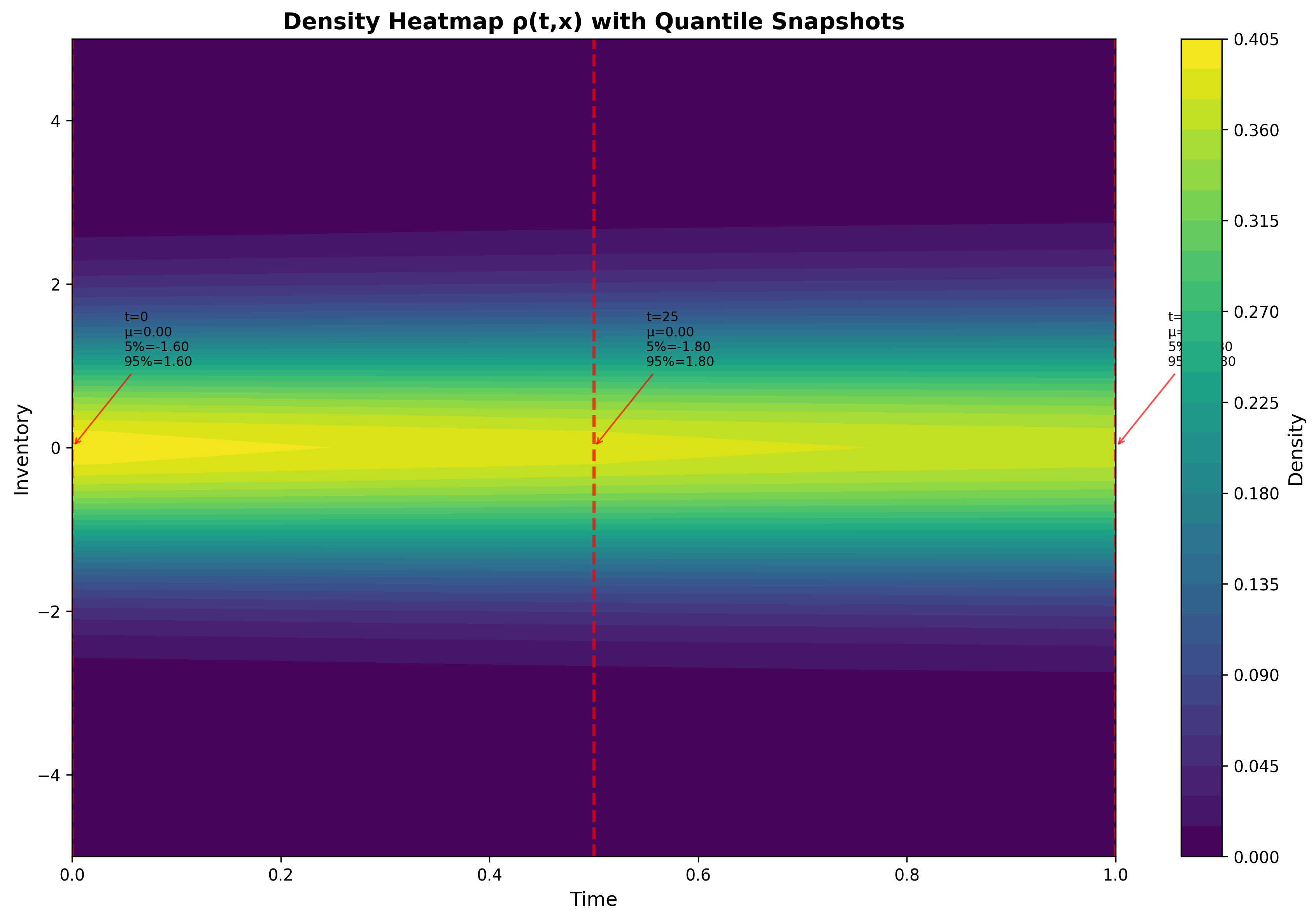
Population Density Heatmap: 2D view of ρ(t,x) showing the crowd's movement toward zero inventory
Mean-field coupling: competition
Naturally, customers route to tighter quotes. A simple, tractable way to encode competition is to make intensities depend on relative tightness: \(\lambda^a\big(\delta^a;\,\bar{\delta}^a_t\big) \;=\; A\,e^{-k(\delta^a-\bar{\delta}^a_t)}, \qquad \bar{\delta}^a_t \;=\; \sum_x \delta^{a*}(t,x)\,\rho(t,x),\) \(\lambda^b\big(\delta^b;\,\bar{\delta}^b_t\big) \;=\; A\,e^{-k(\delta^b-\bar{\delta}^b_t)}, \qquad \bar{\delta}^b_t \;=\; \sum_x \delta^{b*}(t,x)\,\rho(t,x).\)
Note (functional form): The form $A\,e^{-k(\delta-\bar{\delta})}$ is invariant to uniform shifts $\delta \mapsto \delta+\Delta$, $\bar{\delta} \mapsto \bar{\delta}+\Delta$. If you want absolute tightness of the crowd to change total flow (e.g. spread compression increases trading), a minimal drop-in is to multiply by a decreasing total-flow term, \(\lambda^a\big(\delta^a;\,\bar{\delta}^a_t\big) = \underbrace{\Lambda_{\text{tot}}\!\big(\bar{\delta}^a_t\big)}_{\text{decreasing in }\bar{\delta}^a_t}\, e^{-k(\delta^a-\bar{\delta}^a_t)}, \qquad \Lambda_{\text{tot}}(\bar{\delta})\;=\;A_0\,e^{-k_0 \bar{\delta}}.\) Alternatively, use a market-share split for relative competition, \(\lambda^a\big(\delta^a;\,\bar{\delta}^a_t\big) = \Lambda_{\text{tot}}\, \frac{e^{-k\delta^a}}{\,e^{-k\delta^a} + (N-1)\,e^{-k\bar{\delta}^a_t}\,}\,,\) which preserves demand allocation while keeping overall flow explicit via $\Lambda_{\text{tot}}$.
Algorithmically we solve a fixed point:
- Guess $\bar{\delta}^a(t)$ and $\bar{\delta}^b(t)$.
- Solve HJB backward to get $V$ and $\delta^{*}$.
- Solve the master equation forward to update $\rho$ and recompute $\bar{\delta}$.
- Repeat 2–3 until $\bar{\delta}$ stabilizes.
Discretization
To solve this system we use a grid: times $t_n=n\Delta t$ and inventories $x_i\in{-X_{\max},\dots,X_{\max}}$.
Backward (HJB) — start from $V(T,x)=-\gamma x^2$. For each step $t_{n+1}\to t_n$, compute $\delta^{*}$ from the closed forms (with finite differences for $V(t,x\pm1)-V(t,x)$), then update $V$ with a stable backward step.
Forward (Fokker–Planck)
\[\rho_{n+1,i} = \rho_{n,i} +\Delta t\,\bigl( \rho_{n,i+1}\,\lambda^{a}_{n,i+1} +\rho_{n,i-1}\,\lambda^{b}_{n,i-1} -\rho_{n,i}\,(\lambda^{a}_{n,i}+\lambda^{b}_{n,i}) \bigr).\]ignoring terms that would step outside the inventory grid (reflective/absorbing behavior as chosen). This conserves probability up to numerical error. We enforce $\rho_{n+1,i} \ge 0$ and renormalise so that $\sum_i \rho_{n+1,i}\,\Delta x = 1$ at each step (numerical mass conservation).
Metrics \(\bar{\delta}^{\,b}(t_n) \;=\; \sum_i \delta^{b*}_{n,i}\,\rho_{n,i}, \qquad \bar{\delta}^{\,a}(t_n) \;=\; \sum_i \delta^{a*}_{n,i}\,\rho_{n,i},\) \(\text{FullSpread}(t_n) \;=\; \bar{\delta}^{\,a}(t_n) \;+\; \bar{\delta}^{\,b}(t_n), \qquad \mathrm{Var}[X](t_n) \;=\; \sum_i (x_i - \bar x_n)^2\,\rho_{n,i},\) \(P\big(|X_{t_n}|<\varepsilon\big) \;=\; \sum_{\lvert x_i\rvert<\varepsilon} \rho_{n,i}, \qquad \partial_x V(t_n,0) \approx \frac{V(t_n,\Delta x) - V(t_n,-\Delta x)}{2\,\Delta x}.\)
Interactive Metrics Table
Metrics Table: Real-time computation of all key metrics
rises as $\lvert x\rvert$ grows; steepens near $T$ (less time to fix mistakes).
Interpreting the dashboard
Value surface $V(t,x)$: deepest near $x=0$ ,safe when flat, rises as $\lvert x\rvert$ grows and steepens near $T$ as there is less time fix heavy position
Value surface $V(t,x)$: deepest near $x=0$ (safe when flat),
Control surface $\delta^{*}(t,x)$: small (tight) where trading is urgent (e.g., long inventory near close); larger (wide) when you want to slow down.
Distribution $\rho(t,x)$: the ridge of the crowd funneling toward zero inventory over time—some finish early, others lag.
Spreads over time: average bid and ask and their difference (full spread) reveal competition’s compression during the session (when using the competition model above; otherwise read as spread dynamics under the chosen policy).
Variance: shows where crowding peaks (often mid-session).
De risk probability: fraction of makers inside $x<\varepsilon$; if it misses a policy target by $T$, increase $\eta$ or $\gamma$.
Marginal cost $\partial_x V(t,0)$: a shadow price for one more unit at flat inventory—useful as a real-time risk budget.
Key formulas at a glance
Poisson intensities \(\lambda(\delta)\;=\;A\,e^{-k\delta}, \qquad \lambda(\delta-\Delta\delta) \;=\; e^{k\Delta\delta}\,\lambda(\delta).\)
Objective
\[J^\pi(t,x) = \mathbb{E}_{t,x}^{\pi}\!\left[ \int_{t}^{T} \bigl(\delta^a\,dN^a + \delta^b\,dN^b - \eta\,X^2\,dt\bigr) \;-\; \gamma\,X_T^2 \right].\]Value function \(V(t,x)\;=\;\sup_{\pi} J^\pi(t,x).\)
HJB \(-\partial_t V = \sup_{\delta^a,\delta^b} \left\{ \lambda^a(\delta^a)\,[\delta^a+V(t,x-1)-V(t,x)] + \lambda^b(\delta^b)\,[\delta^b+V(t,x+1)-V(t,x)] - \eta\,x^2 \right\}, \qquad V(T,x)=-\gamma x^2.\)
Optimal quotes \(\delta^{a*}\;=\;\frac{1}{k}-\big[V(t,x-1)-V(t,x)\big], \qquad \delta^{b*}\;=\;\frac{1}{k}-\big[V(t,x+1)-V(t,x)\big].\)
Population (master equation) \(\partial_t \rho = \rho(t,x+1)\lambda^a\!\big(\delta^{a*}(t,x+1)\big) + \rho(t,x-1)\lambda^b\!\big(\delta^{b*}(t,x-1)\big) - \rho(t,x)\big(\lambda^a\!\big(\delta^{a*}(t,x)\big)+\lambda^b\!\big(\delta^{b*}(t,x)\big)\big).\)
Mean field \(\bar{\delta}^a_t=\sum_x \delta^{a*}(t,x)\,\rho(t,x), \qquad \bar{\delta}^b_t=\sum_x \delta^{b*}(t,x)\,\rho(t,x).\)
Consistency checks used in the code.
- Spread identity: we verify $\mathbb{E}[\delta^a+\delta^b] = \mathbb{E}[\text{ask} - \text{bid}]$ to numerical precision.
- Intensity monotonicity: $\lambda(\delta)$ decreases in $\delta$.
- Mass conservation: $\sum_i \rho_{n,i}\,\Delta x = 1$ at each time.
Conclusion
The fair opens. You choose prices (quotes). Tight prices attract buyers but may pile up baskets; wide prices keep you safe but slow you down. The crowd’s average behavior feeds back into your fortunes: if everyone tightens, bargains abound and your edge shrinks; if the crowd widens, your caution looks wise.
The mathematics: Poisson intensities, a clean HJB with closed-form optimal quotes, and a forward equation for the population—turns this story into a solvable loop that yields policy maps and risk-aware schedules a desk can actually use.